data of  ,
,  is the mean value of sample data;
  is the covariance matrix of samples
  ,
,  is the eigenvector matrix of
  ;
;  is the multivariate kernel function;
  is the window width matrix, the selecting principle of
  is to minimize the mean square error of calculation results; the kernel density estimation points
  ,
,  is a vector which is the independent variables of kernel density estimation function, herein,
  is the vector
  , which is obtained from the transformation
  based on the structural output responses
 .
.
3.3 Maximum likelihood estimation
The maximum likelihood estimation is implemented aiming at the output response of the structural model, and the parameter satisfying the probability distribution density is estimated. The parameter with the greatest possibility  is taken as the estimation value of the real parameter
 . Since the log likelihood function is easier to calculate, the kernel density estimation function in Eq.(31) is then expressed as
 (32)
(32)
whereby  is a super parameter, i.e.,
  ,
,  is the mean variance of Gaussian random field and
  is the correlation length of random field; simulation output response
  ,
,  is the output response of the model with super parameter
  , the covariance matrix of samples
  is
is  and
and  is the eigenvector matrix of
  ;
;  ,
,  is the output responses of tests and
  means the number of test points. According to the assumption of kernel function of multivariate Gaussian distribution [8], the window width is taken as
 (33)
(33)
whereby  is the eigenvalue matrix of covariance matrix
  .
.
The Gaussian kernel function is chosen as
 (34)
(34)
The maximum likelihood estimation method is used to quantify the distribution parameters of the test samples, i.e. assuming a group of parameters  , the output responses of these parameter samples are then taken as the model samples. The probability distribution density function of the output responses is then obtained by using the kernel density estimation aiming at these output response values based on Eq.(31), and the maximum likelihood estimation function
  can be computed by inserting the output responses from both test samples and model samples into Eq.(32) and finally the parameter
  can be estimated which is corresponding to the maximal value of
  , so as to verify whether it is the input parameter of test samples.
4. Examples
4.1 I-beam with one-dimensional random field
Fig.3 is a simply supported steel beam with the section of I-beam and the length of the beam is 1m. The inertia moment  , sectional area
  , mass density per unit length
  and material modulus of elasticity of 210
 . The beam is meshed into 60 beam elements as shown in the right figure of Fig.3.
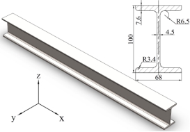
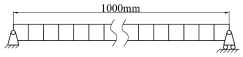
Fig.3 No. The geometric dimensions of 10 I-beam (left) and its meshing elements (right)
Suppose that Yang��s modulus of material  is random field and its mean value is
  , and the covariance function is taken as
  . Then K-L expansion of
  in every element from Eq.(1) is

From Eq.(35), the random field of  is represented with its mean variance
  and correlation length
 , i.e., the super parameter
  is the output parameter of test samples and model samples,
  . In the following, the random field of
  is quantified with numerical tests. Based on Section 3.1, the first eight-order natural frequencies can be solved for every I-beam, and the natural frequency matrix can then be formed as
  .
.
Given an input parameter  , and natural frequency matrix of 500 beams
  are considered as the test data samples. Moreover, the other super parameters
 are chosen, and the detailed values of parameters are
  and
and 

 . The natural frequencies of 100 beams for each super parameter
  form a model matrix sample
  , and there are in all
  beams and 100 model matrix samples
  . In the following, the kernel density estimation and maximum likelihood estimation will be implemented aiming at natural frequency, and the identifiability of super parameter
  and the effectiveness of random field model will be verified.
4.1.1 Test data analysis
For four super parameters of Young��s modulus  ,
,  ,
,  and
and  , the random process distribution of
  on 10 beams are demonstrated in Fig.4, in which every curve denotes the value of
  on the beam and reflects the randomness of values of
  on every point of the beam. From Fig.4, it can be seen that values of the random field of
  fluctuates around its mean value 210GPa; the fluctuation along the longitudinal axis reflects the magnitude of variance and the variation of variance with the axial dimension of the beam; just as the meaning of super parameter
  and
and  , the influence of
  on the random distribution of
  is much greater than that of
  . In the case of the same super parameter, 10 curves in each figure, i.e. random field distribution of
  , are very different, but the general distribution law is similar because of the same super parameter in each figure. Also it can be ovserved from Fig.4 that
  directly affects the randomness distribution of every element in the beam, that is, the larger the correlation length is, the more acute the value fluctuation of
  along the direction of beam length is.
Based on the conclusions of Fig. 4, the super parameter  will be used in the subsequent analysis.
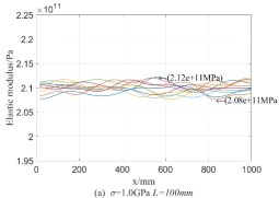
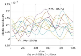
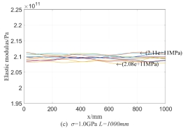
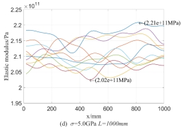
Fig.4 random field of Yong��s modulus  in the beam
4.1.2 one-dimensional kernel density estimation
In order to verify the applicability of the super parameter  , the test samples
  and model samples
  of the second-order natural frequency of the beam are chosen and used for the one-dimensional kernel density estimation of the single parameter of the second-order natural frequency.
Firstly, when taking  and
and  , which form 10 super parameters
  . For 100 beams corresponding to each
  , the second-order natural frequency is solved and the model sample
  is formed. Then taking 100 beams with super parameter
  and
and  , the second-order natural frequencies of 100 beams construct test samples
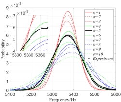
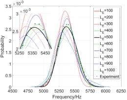
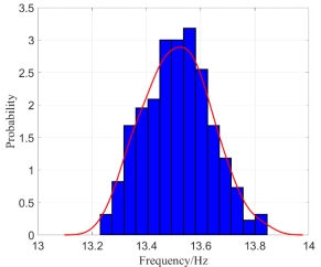
  . Fig.5(a) displays the one-dimensional kernel density estimation of the structural second-order natural frequency calculated based on
  and
and  . From Fig.5(a), it can be seen that distributions of natural frequencies of model samples become more and more concentrated with the decreasing
  , and the distributions are very close to each other when
  of both test samples and model samples is
  .
.
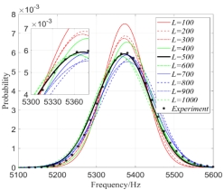
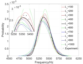
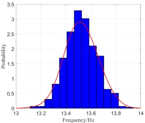
In the same way, when  and
and  , the second-order natural frequencies of 100 beams form the model samples data
  ; then taking the test sample data
  when
when  and
and  , one-dimensional kernel density of
  is estimated based on
  and
and  as shown in Fig.5(b). From Fig.5(b), the distribution of
  of model samples become more and more concentrated with the decreasing correlation length ; the distributions of
  of model samples and test samples are closest when correlation lengths of two types of samples are equal. Once again, Figure 5 shows that the influence of
  on the fluctuation of kernel density is greater than that of correlation length.
(a)  (b)
(b) 
Fig.5 one-dimensional kernel density distribution function of  when only considering random field of
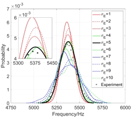
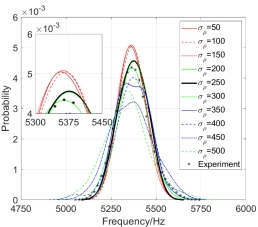
Similarly, considering that the Yong��s modulus  and mass density
  are random fields varying with the change of space size, the super parameters are taken as
  and 100 beams are used. The one-dimensional kernel density of
  is estimated again, where
  and
and  . The left figure is the one-dimensional kernel density distribution function estimated of
  when
when  but
but  changes, and the right figure is the one-dimensional kernel density estimated of
  when
when  but
but  varies. When
  , in Fig.5(c),
  changes but
  =
= ; and Fig.5(d) is the resutls estimated when
  but
but  changes.
It can be seen from the Fig.6 that the influence of  and
and  on the kernel density distribution function is significantly greater than that of
  and
and ; when other parameters are fixed but
  and
and  change respectively, the influence of
  on the kernel density distribution function is greater than that of
  ; when other parameters are fixed but
  and
and  change respectively, the influence of
  on the kernel density distribution function of
  is greater. In general, the mass density random field has a greater influence on the kernel density distribution function of
  than the Young��s modulus random field.
(a)  (b)
(b) 
(c)  (d)
(d) 
Fig.6 one-dimensional kernel density estimation of the second-order natural frequency when considering Young��s modulus and mass density random fields
4.1.3 Multidimensional kernel density estimation and maximum likelihood estimation
In order to more accurately verify the validity of the random field model and the identifiability of the super parameters, it is necessary to further estimate the multi-dimensional kernel density probability distribution function of the structure output responses, and then to carry out the maximum likelihood estimation to obtain the super parameter corresponding to the maximal value of likelihood function.
When considering Young��s modulus random field, based on 100 model matrix samples  from
from  beams and test samples
  from 500 beams, the 8-dimensional kernel density of the first 8-order natural frequencies of the beam is estimated, and then the parameter
  is estimated by the maximum likelihood based on Eq.(32), in which
  and
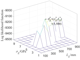
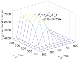
and  are composed of the first 8-order natural frequencies of the structure. Because the values of probability density function of some points are small, in order to avoid the calculation value of likelihood function is 0, it is necessary to take the logarithm of the value of probability density function firstly and then implement summation. The obtained log likelihood function is illustrated in Fig.7.
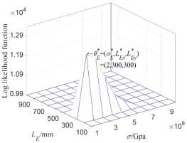
Fig.7(a) is the log likelihood function  of the first 8 natural frequencies when the super parameters of the test data samples are taken as
  . It can be seen that when
  is taken as its maximum value, the parameter
  of the corresponding point is
  , which shows that the random field model introduced can identify the model parameter very well, and the random field model is reliable.
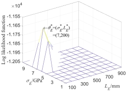
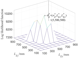
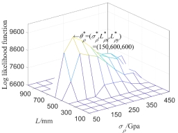
In Fig.7(b), based on Eq.(32), a group of super parameter values of test samples are randomly taken as  , and the multi-dimensional kernel density probability distribution function is estimated for the first 8 natural frequencies, and then the maximum likelihood estimation is carried out. The estimated parameter results
  are slightly different from the original super parameter
  . This is because the amount of the model samples cannot be taken as infinite and the estimation accuracy of the input parameter of test samples is obviously limited by the amount of the model samples, but the peak value of likelihood function can still be obtained near the parameter
  , i.e.,
  .
.
(a) (b)
(b) 
Fig.7  of 8-dimensional kernel density distribution function of the first 8 orders natural frequency when only considering random field of
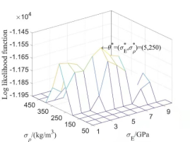
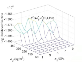
When considering the random fields of both Yong��s modulus  and mass density
  at the same time, the input parameters of the test samples are taken as two groups respectively:
  ,
,  and
and  ,
,  . The correlation length of two random fields is fixed, that is,
 , the mean variances
  and
and  are estimated when the likelihood function
 are taken as its maximal values. It can be seen from Fig.8 that the super parameter at the maximum value point of
  is the same as the input parameter by using the maximum likelihood estimation for the first 8 order natural frequency of the structure.
(a)  (b)
(b) 
Fig.8  of 8-dimensional kernel density distribution function of the first 8 orders natural frequencies when both
  and
and  are random fields
4.2 Example 2: plate with two-dimensional random field
Fig.9 shows a square steel plate fixed at one end, with a thickness of 0.01m, the mean values of mass density and Yong��s modulus are  and
and  . The plate is meshed into 400 rectangular plate elements.
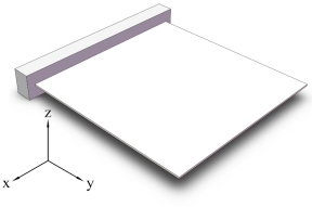
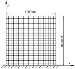
Fig.9 the plate fixed at one end (left) and its mesh elements (right)
Considering Yong��s modulus  of the plate is two-dimensional random field,
  is then expanded with K-L expansion as follows

 (36)
(36)
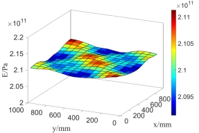
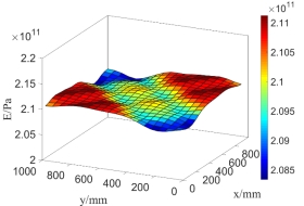
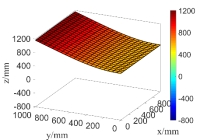
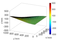
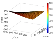
Fig.10 Random field distribution of  in the plate in the case of
  elements (left) and
 elements (right)
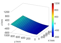
Taking the super parameter of random field  ,
,  , as the input parameter of test samples and model samples. When the plate is meshed into different amounts of elements, the distribution of random field
  in the plate is displayed in Fig.10.
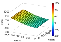
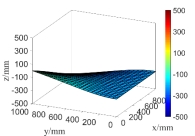
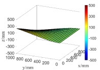
Also, only considering mass density as random field,
  is expressed with the two-dimensional K-L expansion as Eq.(37), whereby its mean value is
  . Taking its super parameter
 and meshing the plate into different amount of elements, the distribution of random field
  in steel plate is displayed in Fig.11.

 (37)
(37)
It can be seen from Fig.10 and Fig.11 that the values of  and
and  fluctuate and vary around the mean values
  and
and  , and the values of
  and
and  randomly distributed in X and Y directions. Moreover, compared with the random distributions of the values at every point for
  and
and  in the plated with 225 meshing elements, the random distributions with 400 elements obviously reflect the real cases better and more accurate.
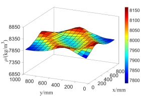
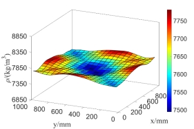
Fig.11 Random field distribution of  in the plate in the case of
  elements (left) and
 elements (right)
When only considering the random field of  , a group of super parameters are taken as
  , and the specific parameter values are
  ,
,  and
and 
 . Taking 100 plates for each super parameter
 , the first six natural frequencies of 100 plates are taken to form the model matrix samples
 . A total of 1000 model matrix samples
  and
and  plates are used. Next, the kernel density estimation and maximum likelihood estimation will be performed on the test data samples based on the model data samples.
Tab.1 The maximum likelihood estimation of test samples when considering random field of material parameter 
|
Input super parameter of test samples of 500 plates

|
The maximal value of log likelihood function 
|
Super parameter estimated from 
|
Mean value and mean variance of the first three natural frequencies obtained from 500 test samples of 500 plates
|
|

|
 
|
 
|
 
|
|

|

|

|

|

|

|

|

|

|
|
(5,500,500)
|
10344.12
|
5
|
500
|
500
|
8.6185
|
0.0581
|
13.5240
|
0.0877
|
51.6952
|
0.3545
|
|
(6,300,700)
|
9190.03
|
6
|
300
|
700
|
8.6159
|
0.0659
|
13.5199
|
0.0969
|
51.6793
|
0.3957
|
|
(2,100,700)
|
13712.95
|
2
|
100
|
700
|
8.6197
|
0.0131
|
13.5254
|
0.0183
|
51.7022
|
0.0776
|
|
(9,430,650)
|
8151.44
|
9
|
400
|
700
|
8.6204
|
0.1083
|
13.5271
|
0.1627
|
51.7069
|
0.6553
|
Herein  and
and  denote the mean value and mean variance of the random variables.
In order to verify the random field model of the plate, the super parameters  ,
,  ,
,  and
and are respectively taken for numerical simulation, and 500 plates are used for the computation of each super parameter. The first six natural frequencies of 500 plates are taken for each super parameter to form the test matrix samples
  ,
, ,
,  and
and  respectively, and then the logarithmic likelihood functions
  are calculated by Eq.(32) and the computational results are listed in Table 1.
From Tab.1, according to the point at which the maximal value of  is obtained, it can be seen that the super parameter of test samples
  can be well estimated by the presented two-dimensional random field model of the plate, which are basically consistent with the input super parameters
  ,
,  ,
,  and
and  of the test samples. Hence, the constructed two-dimensional random field model is reliable. Similarly to the one-dimensional random field model of I-beam, the amount of model sample groups may not be infinite, and the estimation accuracy of test sample parameter is limited by the amount of the model samples. When the maximum likelihood estimation method is used to estimate the test samples with input parameter
 , the input parameter of test samples can still be estimated comparatively accurately.
Furthermore, the super parameters of  and
and  are respectively taken as
 and
and 
 . When
  is taken as
  ,
,  and
and  respectively, super parameters of the test samples are taken as
  and
and  , the two-dimensional kernel density distribution function of the second-order natural frequency
  of test samples is estimated as shown in the left figure of Fig.12.
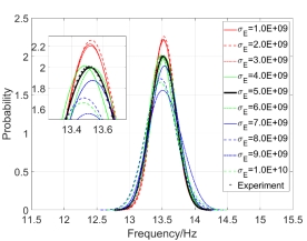
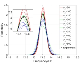
Fig.12 The one-dimensional kernel density estimation of  when both
  and
and  are random fields
The histograms of  when both
  and
and  are random fields:
  elements (left) and
 elements (right)
Similarly, super parameters of  and
and  are
are  and
and  , and respectively taking
  as
as  ,
,  , ��,
, ��,  in the computing, and then taking super parameters of test samples
  and
and  , the two-dimensional kernel density distribution function of
  is estimated and shown in the right figure of Fig.12.
Fig.12 shows again that random field of  has a more influence on the kernel density distribution function of structural natural frequency than the random field of
  .
.
(a)  (b)
(b) 
Fig.13 The log likelihood function  of the first 6 natural frequencies when inputting different super parameters of random field
In addition, fixing mean variance of super parameter  , i.e.,
  , then taking correlation length
  and
and  as variables, the variation of likelihood function of natural frequency with
  and
and  are shown in Fig.13 (a). Similarly,
  is obtained in Fig.13(b) when super parameters of test samples are
  and
and  . In Fig.13, the plate is meshed into 400 elements.
It can be seen from Fig.13 that the super parameters  obtained corresponding to the maximal value
  are respectively
  and
and 
 ; based on the multi-dimensional kernel density estimation, the super parameters of test samples when the maximum likelihood function is obtained can be accurately estimated, and the estimated super parameters are very close to the input parameters of the test samples, which verifies the validity of the constructed model.
In the same way, when only the mass density is random field and the input super parameters  of the test samples are
  and
and 
 respectively, the log likelihood function obtained based on the first six natural frequencies of the plate are displayed in Fig.14.
(a)  (b)
(b) 
Fig.14 The log likelihood function  of the first 6 natural frequencies when inputting different super parameters of random field
Fig.15 shows the first six order random natural modes of the steel plate when only considering  as the random field, and the super parameter after K-L expansion is
 .
.
(a) the first order natural mode

(b) the second order natural mode
Fig.15 The random natural modes of the steel plate when only considering random field of 
When considering random fields of  and
and  and taking their super parameters as
  and
and 
 , the first 6random natural modes are illustrated in Fig.16.
The norms of the first 8 order natural modes are computed and listed in Tab.2 for different random models so as to compare the influences of different random cases on the structural natural modes.


(a) the first order natural mode

(b) the second order natural mode
Fig.16 The first 6 order natural modes of the plate when considering random fields of both  and
and 
From Fig.15 and Fig.16 as well as the computational results in Tab.2, it can be seen that the natural modes only considering random field of  are very close to those simultaneously considering random fields of
  and
and  except for the fifth natural mode, that is,
Tab.2 Comparison of the norm of natural modes for different random models
|
Computational results
Random models
|
Norm of random natural modes
|
|

|

|

|

|
|

|

|

|

|

|

|

|

|
|
Deterministic model
|
6342.80
|
0
|
1635.00
|
0
|
399.12
|
0
|
296.67
|
0
|
|
Random field of 
|
6346.67
|
94.82
|
1635.12
|
6.56
|
399.25
|
3.73
|
357.71
|
1010.50
|
|
Random fields of  and and
|
6347.82
|
134.34
|
1635.43
|
7.71
|
399.21
|
3.98
|
477.17
|
1249.14
|
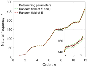
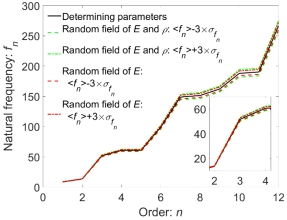
Fig.17 Random natural frequencies for different random models: experimental samples (left) and  (right)
Tab.3 Comparison of the norm of natural modes for different random models
|
Computational results
Random models
|
Norm of natural modes
|
|

|

|

|

|
|

|

|

|

|

|

|

|

|
|
Deterministic model
|
8.62
|
0
|
13.52
|
0
|
51.67
|
0
|
60.68
|
0
|
|
Random field of 
|
8.62
|
0.0583
|
13.53
|
0.0885
|
51.69
|
0.3580
|
60.69
|
0.3914
|
|
Random fields of  and and
|
8.62
|
0.0906
|
13.52
|
0.1321
|
51.65
|
0.5651
|
60.62
|
0.6235
|
5. Conclusions
The super parameter model based on random field theory can represent the uncertainty of structure well, and reflect the uncertainty and spatial correlation of structure parameters. Also the super parameter model presented can describe the randomly varying characteristics of actual structure parameters. The example shows that the super parameters of the model can be quantified by the output response of the structure, i.e. the natural frequency of the structure, and the mean variance and autocorrelation distance of the super parameter of the structure can also be obtained, which is very important to the application of random field in the engineering. The proposed method can be extended to apply to other parameters, and can also be used to establish and quantify the super parameter model of random fields for other material parameters or structural parameters. The applicability and effectiveness of the proposed computational framework are evidently demonstrated through the numerical investigations on various practically motivated engineering structures.
References
[1] ����ˮ,�����,�Ŷ���.������������۵Ľṹ��ȷ���Ա���������[J].����ҵ�Զ���,2015,(��15��).
[2] �׳���,�ź���.��ȷ����ת��ϵͳ���������Ԫ��ģ����Ӧ����[J].����ѧ�����ѧ��,2012,(��3��).
[3] FENG X, LU Z X, YANG Z Y, et al. Analysis on the variances of material and structural properties based on random field theory[J]. Probabilistic Engineering Mechanics.2011(26):222-230.
[4] BETZ W, PAPAIOANNOU I, STRAUD D. Numerical methods for the discretization of random fields by means of the Karhunen�CLo��ve expansion[J].Computer Methods Applied Mechanics and Engineering.2014(271):109-129.
[5] Roger G. Ghanem, Pol D. Spanos. Stochastic finite elements:a spectral approach[M]. Dover Publications, 2003
[6] ����������. ��е��. ��ѧ����������, 1985.06.
[7] ���ڽ�,�����.����Ԫ����������[M].�廪��ѧ������,2009
[8] SOIZE C. A computational inverse method for identification of non-Gaussian random fields using the Bayesian approach in very high dimension[J].Computer Methods Applied Mechanics and Engineering,2011(07).
, Uncertain dynamic characteristic analysis for structures with random fields
Changhu Zhou1, Juan Ma*1, Changping Dai1, Jean W Zu2
1Key Laboratory of Electronic Equipment Structure Design, Ministry of Education, Xidian University,
Xi��an 710071, P. R. China
2 Department of Mechanical Engineering, Stevens Institute of Technology, 1 Castle Point Terrace, Hoboken, NJ 07030, New Jersey, USA
Abstract: This work presents a robust non-deterministic free vibration analysis for engineering structures with spatially dependent uncertain system parameters. For this, considering the randomness and spatial correlation of structural physical parameters, a super parameter model based on the random field theory is proposed to represent the random uncertainty of parameters, and the stochastic dynamic characteristics of different structural systems are then analyzed based on the presented super parameter model. Firstly, the Gauss random field theory is used to describe the uncertainty of structural material parameters, and the random parameters are then characterized as the standard deviation and correlation length of the random field, and the random field parameters are then discretized with the Karhunen-Loeve expansion method. Moreover, based on the discretized random parameters and finite element method, the structural dynamic characteristics analysis is addressed, and the probability distribution density function of the random natural frequency is estimated based on the multi-dimensional kernel density estimation method. Finally, the random field parameters of the structures are quantified by using the maximum likelihood estimation method so as to verify the effectiveness of the proposed method and the applicability of the constructed model.
Keywords: free vibration; random field; Karhunen-Loeve expansion; multi-dimensional kernel density estimation; random dynamic characteristic
1 Introduction
Structural dynamic characteristics such as the natural frequency, as a key indicator for the vibrational performance of engineering structural systems, has been extensively studied in the past decades. With the aid of finite element method (FEM), such essential dynamic characteristic of engineering structures can be adequately obtained by solving the generalized eigenvalue and eigenvector problems. Despite that the system variables of the concerned structures are widely assumed as deterministic, it has been illustrated that the fluctuation, or so-called uncertainties, of these parameters inherently associates with the structures as well as the modelling process [1�C3]. The complexity of the actual structural material properties and various random errors during the manufacturing process will cause the uncertainty of the structural parameters, such as the vibration of the machine tool, the random variation of the temperature during the processing, etc., which will result into the uncertainty among a group of structural parts with the same nominal size that are manufactured with the same material and the same processing method, and ultimately lead to the random fluctuation of material properties around the mean value and a certain correlation between the fluctuation and machining dimension direction. In addition, a group of structural members with the same nominal size, because of the uncertainty of their material parameters, may have the similar but different dynamic characteristics. The existence of such uncertainties potentially affects the credibility of the analyzing results of the dynamic behaviors of the structural systems, which leads to the indispensability of developing an uncertain free vibration analysis framework for a more effective and meaningful prediction on the structural natural frequencies as well as other dynamic characteristics [4�C6]. So it is urgent to build an effective model to represent the uncertainty of structural parameters.
Conventionally, the uncertain free vibration analysis is initialized by implementing probabilistic/stochastic approaches, which are established on the solid theoretical foundation of probability or statistics. In structural engineering, the random eigenvalue problem is adequately addressed by the stochastic finite element method (SFEM) by incorporating the probabilistic strategies within the FEM [7�C10]. Accordingly, the concerned uncertainties of the structural system parameters are modelled as stochastic parameters with the pre-defined statistical information such as means and standard deviations. With the progressive development of uncertainty analysis, SFEM has been escalated with the consideration of the spatial dependency of uncertain system parameters by incorporating the theory of random field. Numerous computational procedures have been developed for solving the random eigenvalue problem [11�C13], as well as other engineering applications [14�C19]. Generally, the implementation of SFEM can be classified into two categories: the simulative approaches (e.g., direct Monte-Carlo simulation (MCS)) which are capable in offering the probabilistic features of the concerned structural responses based on the collection of samples obtained from the simulation [20�C24]; and the non-simulative strategies which approximate the statistical characteristics of the structural system outputs by implementing various numerical methods [25�C29]. Admitting the universal application of SFEM, it is worthy to pointing out that the creditability of such stochastic procedures is conditional to the availability of the statistical information of the concerned uncertainties in practical engineering applications [30�C32].
����ˮ��[1]����һά��˹�����ģ�ͣ�������K-Lչ�����������ɢ������Ԫģ�ͣ��������������Ķ������ԣ��׳����[2]��һά�����������ʾ��ĵ���ģ��������ģ�����ܶȵȲ������о��˲�ȷ����ת��ϵͳ���������Ԫ��ģ��������Ӧ������Feng X��[3]���û�����������۵��������Ԫ���о��ṹ������ѧ���ܵı仯���ɣ�����һά����������ĵ���ģ�����غɺ������ܶȽ��б������о��˼�֧���Ķ���ѧ���ԡ�
At present, the research on the characterization of structural uncertainty and the modification of structural parameters mainly focuses on the expansion of some structural or material parameters, such as elastic modulus, the moment of inertia, thickness, etc., and input the mean values and mean variances of these discrete random variables into the structural system for an uncertainty analysis. These constructed models are not very complex, and can not accurately reflect the real uncertainty of the actual structure although various effective methods can be used for the stochastic finite element analysis. In fact, there are many factors that affect the uncertainty of structural material parameters, resulting in the random distribution of material parameters in the structural space. For example, manufacturing processes can easily lead to the spatial variations of the load and the material properties such as moduli and density. When rolling steel plates, the runout of the rolling head presents a trigonometric function law, which will inevitably lead to the uneven thickness of the structure and then the randomness of the physical parameters. Accordingly, the randomness of Young's modulus and mass density of the structure is closely related to the spatial size of the structure. In order to fully and objectively study the influence of the key random parameters on the structural analysis, it is very crucial to introduce random field model to describe the spatial correlation of structural material parameters and then address the structural dynamic problem.
Aiming at the uncertainty of structural material parameters, a method of structural dynamic characteristics analysis based on random field theory and the corresponding verification method are presented. Firstly, the uncertainty of structural material parameters is represented by the super parameter model of random field theory, and the uncertainty of random field structural parameters is quantified with the random field model based on Gauss kernel function. Then, the simulation and discretization of the super parameter model of random field are implemented with Karhunen-Loeve expansion method, and the dynamic characteristics of structure are analyzed in the frame of finite element method, followed by the acquisition of the probability distribution density function of the natural frequency by using the multi-dimensional kernel density estimation method. Afterwards, the input parameters of the model are quantified by the maximum likelihood estimation method after comparing the experimental results with the simulation results. Finally, two examples are used as one-dimensional and two-dimensional cases of random fields to verify the applicability and effectiveness of the proposed method.
The remainder of this paper is organized as follows. In Section 2, a brief summary of the concept of random field and the adopted discretization scheme are provided. For non-stochastic representation of spatially dependent uncertainties, the interval field model and the implemented discretization method are illustrated in Section 3. Then, the extended hybrid uncertain eigenvalue problem which encloses both the random and interval fields as well as the proposed computational framework for analysing the hybrid uncertain natural frequencies of structures are comprehensively introduced in Section 4. Furthermore, two practically motivated numerical examples are investigated by the proposed approach and then critically compared with computational exhausted simulation approach in Section 5. Finally, some concluding remarks are drawn in Section 6.
2 Representation of the uncertainty with random field
The errors of machining, heat treatment and material itself will lead to the uncertainty of structures. These errors are usually small and independent. According to the central limit theorem, i.e., the distribution of a large number of independent and small random variables follows the Gaussian distribution, the assumption of Gaussian distribution is easy to calculate and the problem can be solved. In this work, Gauss random field model is used to describe the uncertainty of material parameters of structure.
2.1 Gauss random field model
Gauss random field has two characteristics: 1) its mathematical expectation  and variance
  are constants independent of position coordinates, i.e.,
  ,
,  , whereby
  is a random number and
  represents a point in space; 2) its autocovariance function is only related to the relative position distance of two points in the random field, but not to the absolute position coordinate of two points, i.e., autocovariance
  , whereby
  is the relative distance between two points, and
  is the autocorrelation function of the random field. In addition, the correlation distance
  is another important parameter of Gaussian random field, which indicates that the parameters within the correlation distance
  have obvious correlation. It can be seen that the key to establish random field is to construct its covariance matrix.
In the frame of finite element, the continuous Gauss random field needs to be discretized into random variable vector for the following structural dynamic analysis. There are several commonly used discretization methods of Gauss random field, i.e., spectrum representation, Karhunen-Loeve expansion (K-L expansion) and so on. Herein, K-L expansion method will be used to discretize random field parameters of structures.
2.2 Karhunen-Loeve expansion
Karhunen-Loeve expansion has been widely applied to the continuous process. Essentially, a random field is decomposed into a series of uncorrelated random variables and certain coefficients such as eigenfunctions and eigenvalues by using the K-L expansion. K-L expansion has the following advantages: it has the characteristics of mean square convergence for any type of random field; compared with other methods, when the finite terms of expansion are the same, K-L expansion has the minimum mean square error [6]. In the K-L expansion, a random field  can be expanded into a group of countable and orthogonal random variables, i.e.,
  can be expanded into a combination of the random scalars
  . The specific development process is as follows [1]:
 (1)
(1)
whereby  is the coordinate of a point in the space��
 is the Mathematical expectation,
  is a random event,
  form a Gaussian random sequence with zero mean and they are uncorrelation to each other,
  and
and  are eigenvalues and eigenfunctions of the autocovariance matrix of random field
  .
.
The key of K-L expansion for a random field is to obtain the eigenvalue and eigenfunction of autocovariance matrix  . Because the covariance matrix of a random field is defined in the regular geometric space domain, the eigenvalues and eigenvectors can be easily obtained. The detailed solution process of autocorrelation matrix
  is as follows [5].
 (2)
(2)
whereby the autocovariance function  is bounded, symmetric and positive definite, which ensures that the eigenvalues and eigenfunctions have the following properties: 1) the set of eigenfunctions
  is orthogonal and complete; 2) for each eigenvalue
  , there are at most a limited number of linearly independent eigenfunctions; 3) there is at most one countable infinite set of eigenvalues; 4) the eigenvalues are all positive real numbers; 5) the autocovariance matrix
  can be decomposed into the following forms:
 (3)
(3)
In the case of one-dimensional random field, in order to solve the eigenfunctions  in Eq.(2), the following autocorrelation kernel function can be used
 (4)
(4)
whereby the correlation length of random field  also reflects the attenuation degree of correlation between two points
  and
and  . Therefore,
  is a function of variable
  and the parameter
 ; the integral area
  in Eq.(2) is a real number interval, and it can be taken as
  . Therefore, Eq.(2) can be converted into:
 (5)
(5)
Eq.(5) is further expanded to obtain:
 (6)
(6)
Finding the first derivative of Eq.(6) to  , yields
 (7)
(7)
Finding the derivative of Eq.(7) to  once again and substituting
  with
with  , the differential equation in general form can be obtained as follows
 (8)
(8)
Let  ��Eq.(8) can be converted into
 (9)
(9)
To solve Eq.(9)��its boundary conditions should be found at first. Substituting  and
and  into Eq.(6) and Eq.(7) respectively and rearranging them, the following boundary conditions can be obtained
 (10)
(10)
 (11)
(11)
In summary, Eq.(2) is transformed into a general differential Eq.(9) and its boundary conditions Eqs.(10) and (11), and the general solution of Eq.(9) is
 (12)
(12)
By substituting Eq.(12) into boundary conditions and then rearranging the equations, yields
 (13)
(13)
Based on Eq.(13), to obtain the solution of differential Eq.(9), namely to get Eq.(12), the following conditions must be met:
 (14)
(14)
Solving Eq.(14) and expressing the solution of the first equation as  ,
,  should be within the interval
  , whereby
  is an even number and it indicates the truncated number during the K-L expansion of Eq.(1). Expressing the solution of the second equation of Eq.(14) as
  ,
,  is within the interval
  . The corresponding eigenfunctions are the following Eq.(15) and Eq.(16)

 (15)
(15)

 (16)
(16)
Furthermore, based on the transformation relation  , the corresponding eigenvalues can be derived as

 (17)
(17)

 (18)
(18)
Based on Eqs.(14)-(16), the beam length  ,
,  and the correlation length
 . When the number of truncations are taken as
  , the eigenfunctions
  are illustrated in the left figure of Fig.1. It can be seen directly that the eigenfunctions are actually a series of trigonometric functions, and their periods and amplitudes are related to the values of the chosen order
  , that is, the larger the value of
  , the smaller the period of
  . Based on Eqs.(17)-(18), when
  ,
,  and
and  , the eigenvalues are shown in the right figure of Fig.(1). It can be seen from Fig.1 that the random field
  is composed of eigenvalues
 and eigenfunctions
 based on Eq.(1), the larger the value of
  in the right figure is, the larger the value of low-order eigenvalues such as
  , and the larger the proportion of low-order eigenfunctions such as
  in
in  as shown in the left figure, so the fluctuation of random field is more gentle.
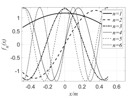
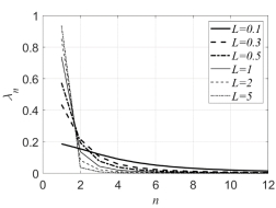
Fig.1 Eigenfunctions (left) and eigenvalues (right) of autocovariance matrix in the case of one dimension
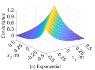
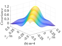
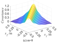
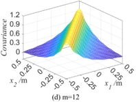
Fig.2 the autocorrelation function  of one-dimensional random variable when
  ,
, and
and 
After the eigenfunctions and eigenvalues of one-dimensional random field are obtained, the autocorrelation function can be obtained based on Eq.(3), i.e.,  . If the length of one-dimensional random field is 1m and the correlation length
  is 0.3m, the autocorrelation function
  is displayed in Fig.2. Fig.2(a) is the autocorrelation kernel function represented by Eq.(4), and Figs.2(b) -2(d) are the autocorrelation functions
  obtained with K-L expansion respectively when the truncation number
  is taken as 4, 8 and 12, whereby
  .
.
It can be seen from Fig.2 that  is more and more close to its autocorrelation kernel function with the increasing
  , that is, the more accurate the autocorrelation function is, the more precise the random field simulation is. Therefore, in the following examples in Section 4, the truncation number
  is selected as 12 with a synthetical consideration of simulation accuracy and calculation workload.
For a two-dimensional Gaussian random field, its eigenvalues and eigenfunctions can be expressed by the product of the eigenvalues and eigenfunctions of two one-dimensional random fields [3] as follows
 (19)
(19)
 (20)
(20)
Substituting Eq.(19) and Eq.(20) into Eq.(1), the following K-L expansion of two-dimensional random field can be obtained
 (21)
(21)
3. Random free vibration analysis of structures with spatial-variant random uncertainty and the quantification of the structural uncertainty
Based on the proposed Gaussian random field model, the uncertainty of structural parameters will be characterized and quantified. In the framework of finite element, the Gauss random field of structural parameters is discretized to every grid element, and the random dynamic characteristics of the structure are calculated. The non-parametric estimation of the dynamic characteristics of the structure will then be implemented by using the kernel density estimation method, so as to obtain the distribution function characteristics of the structural random dynamic characteristics. Finally, the distribution characteristics of the output responses from the test and simulation will be compared with each other, and the distribution parameters of the model will be quantified with the maximum likelihood estimation.
3.1 The analysis of structural dynamic characteristics with random field
Considering that the Young's modulus of the structure is a Gaussian random field, the random field is discretized based on Eq.(1) and then substituted into the following element stiffness matrix and element consistent mass matrix
 (22)
(22)
 (23)
(23)
whereby  is the geometric matrix,
  is the shape function matrix;
  is the integral domain,
  is the unit length for the bar element and beam element, and
  is the unit area for the plate and shell elements;
  is the material density;
  is the elastic matrix shown in Eq.(24) for the beam element,
  is the inertia moment of the beam;
  is the bending stiffness matrix in Eq.(25) for the thin plate element,
  is the Poisson's ratio of the material.
 (24)
(24)
 (25)
(25)
The total stiffness matrix  and the total mass matrix
 of the structural system can be obtained by assembling element stiffness matrix and the element mass matrix and then substituting the boundary conditions of nodes into them. Generally, the vibration that causes damage to the structural system is low-frequency vibration, so in the subsequent analysis, only the low-order natural frequency of the system is considered in this work, and the matrix iteration method is used for solution, so as to quickly obtain the low-order natural frequency of the system and its corresponding vibration mode [6].
Suppose that the structural system represented by the stiffness matrix  and the mass matrix
  is a positive system with
  degrees of freedom, the free vibration equation of the structural system described with the flexibility matrix is as follows:
 (26)
(26)
Let the solution of Eq.(26) be  . Substituting the solution
  into Eq.(26), the following mode equation of system is
 (27)
(27)
Let ��Eq.(27) can be converted into
 (28)
(28)
For the first order eigenvalue  , the relation holds, i.e.,
  . Based on this relationship, the matrix iteration method is used to carry out iteration, and the maximal eigenvalue
  and the corresponding eigenvector
 can be obtained. The specific iteration steps are as follows
1) Taking any normalized mode shape  as the initial solution vector and carrying out the first iteration according to the formula
 , whereby the first components in both
  and
and  are normalized to 1.
2) If  , assigning
  to
to  as the trial solution vector, and repeating the step 1) until the k-th iteration meeting
  , it indicates that the iteration converges if
  , then
  and
and  . It should be noted that the ideal results
 actually can not be obtained in the actual iteration process due to the existence of errors, but it also means the convergence of iterations that the result takes on such an inequality, i.e.,
  , whereby err is the selected error threshold.
To solve the second order and higher order eigenvalues and eigenvectors, the dynamic matrix  needs cleaning, that is,
  needs modifying by using the orthogonality of the main mode and the components of the first
  -order main modes in
  should be cleared, so as to obtain the
  order iterative dynamic matrix. According to the projection theorem of functional theory, the cleaning matrix to be used is
 (29)
(29)
whereby  . Let the dynamic matrix before and after cleaning is
  and
and  ��the specific process of cleaning is
 (30)
(30)
The  order eigenvalue of the system
  and its corresponding eigenvector
  can be obtained by the operation of cleaning for
  mentioned above iterative calculation, and the
  order natural frequency of the system can also be obtained, i.e.,
  .
.
3.2 multidimensional kernel density estimation
Maximum likelihood estimation provides a method to evaluate model parameters with given observation data, i.e., by observing the results of many tests, the parameter can be found that can make the probability of sample occurrence the maximum. Since the distribution characteristics of the output response of the model are unknown, it is necessary to make nonparametric estimation for the probability distribution of the output response. Herein, nonparametric estimation for the probability distribution of the output response is implemented with the multi-dimensional kernel density estimation method.
When the structural parameter is random field, the natural frequency  (
( ) of the model is also random variable. Suppose that natural frequencies are independent and identically distributed random variable, so that the multidimensional kernel density of its distribution density function is estimated as [8]:
 (31)
(31)
whereby  ,
, 
 are the sample
